-
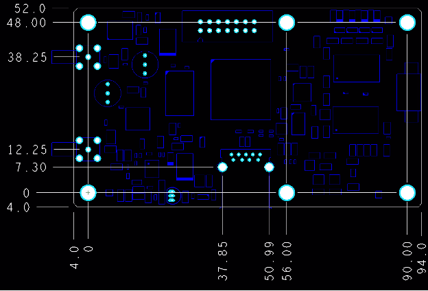
Tolerances and Dimensions for PCB Fabrication
The tolerances decide what actually ships. READ MORE...
-
How to Avoid 'Ghost Manufacturing'
Hidden subcontracting can expose providers to latent quality risks. READ MORE...
-
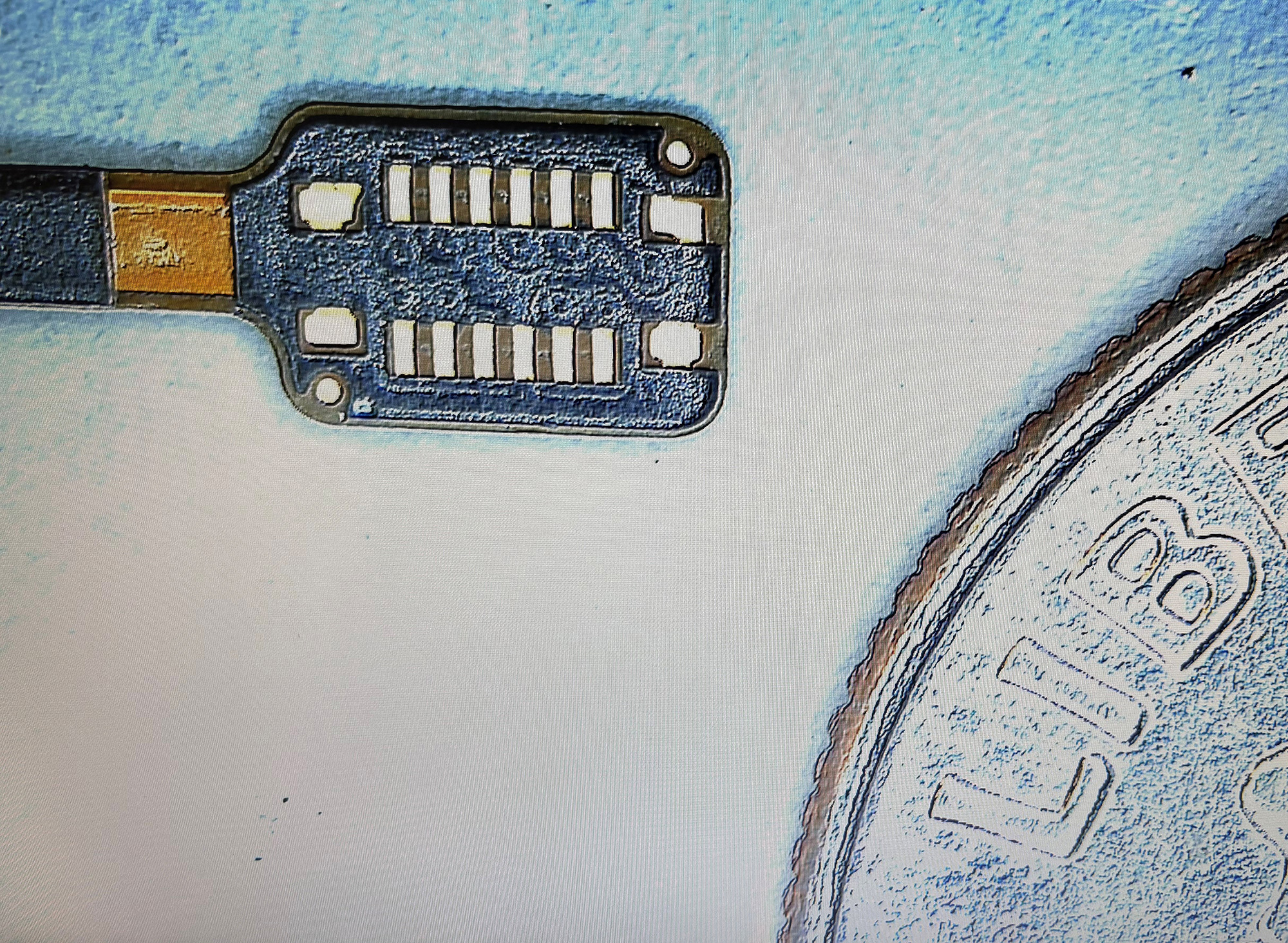
Flex Circuits for Use in Catheters
Long, narrow flex circuits push manufacturing limits. READ MORE...
-
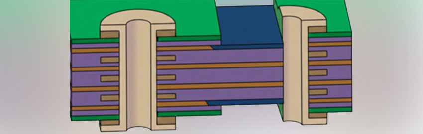
A Guide to Flexible and Rigid-flex PCBs.
What is a flex PCB? READ MORE...
-
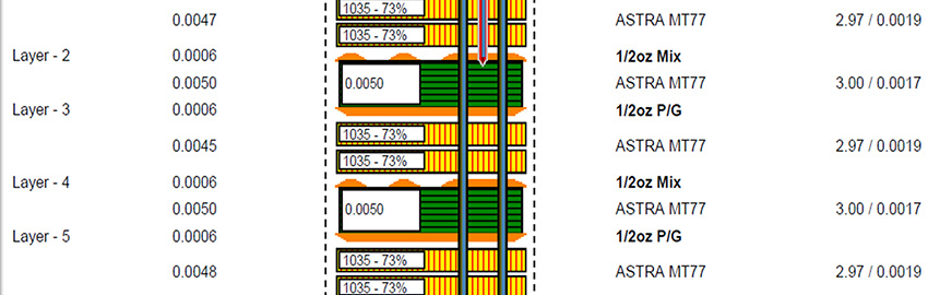
UHDI Solder Mask Considerations
Can solder mask tolerance follow UHDI's lead? READ MORE...
Homepage Slideshow
Tolerances and Dimensions for PCB Fabrication
The tolerances decide what actually ships.
How to Avoid 'Ghost Manufacturing'
Hidden subcontracting can expose providers to latent quality risks.
Flex Circuits for Use in Catheters
Long, narrow flex circuits push manufacturing limits.
A Guide to Flexible and Rigid-flex PCBs.
What is a flex PCB?
UHDI Solder Mask Considerations
Can solder mask tolerance follow UHDI's lead?
https://pcdandf.com/pcdesign/index.php/editorial/menu-features/19210-uhdi-solder-mask-considerations


 Ten steps for achieving good design for excellence.
