Is trace temperature tied to frequency?
In previous articles1 we have written on predicting PCB trace temperatures through the use of computer models in particularly TRM (Thermal Risk Management)2. Here, we will apply TRM to the problem of estimating how AC currents behave on PCB traces, and then verify the models with empirical testing.
High-power, low-frequency currents are sometimes found in relay and control circuits. High-frequency, high-power currents are not terribly common, and usually apply to specialized applications.
Basic Models
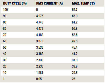
One relatively simple way to utilize TRM is to construct a basic model3 of a trace and apply the appropriate current to it. The trace model we have chosen is the same trace we used in our empirical via paper,4 a 27 mil wide, 2.9 mil thick trace on a dielectric with known thermal conductivity (0.7 W/m-K), mass density (2000 kg/m³) and specific heat capacity (900 J/kg-K). We will apply 5.0As DC to the trace as a reference. We will then assume the applied current is an AC square pulse with a varying duty cycle. The correct equivalent DC current for each duty cycle is the effective RMS current (for a square wave), given by the formula RMS = 5 * SQRT (DCy), where DCy is the duty cycle expressed as a fraction. TABLE 1 provides the detailed equivalent currents and the maximum temperatures from the TRM model for that equivalent RMS current. (These data calculations include effects of the thermal coefficient of resistivity.5)
Table 1. Equivalent RMS Currents and TRM Temperature Calculation
The result is a linear curve, as shown in FIGURE 1.6 The maximum trace temperature is 65.7˚C, with 100% duty cycle (i.e., direct current). It declines in linear fashion to the ambient room temperature at a duty cycle of zero (i.e. no current). The ambient temperature is set to 26˚C in this model for reasons that will be clearer below.
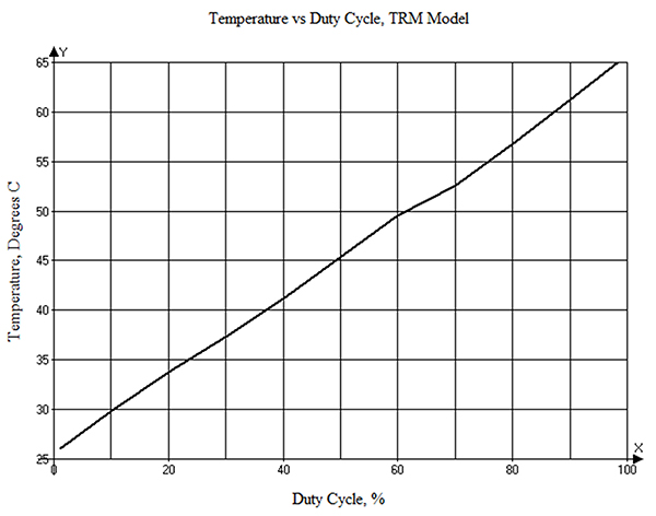
Figure 1. Trace temperature in our model from a 5.0A pulse as a function of duty cycle.
FIGURE 2 illustrates a graph of temperature vs. time for the 5.0A DC current (black line) and for 3.536A DC (dotted red line), which is the RMS-equivalent current for the 5.0A current at a 50% duty cycle. These curves rise asymptotically to the values of 65.7˚C and 45.4˚C, respectively, as expected. The scale on the right-hand axis is the equivalent RMS current (A) that will lead in the long-term to the corresponding temperature on the left axis.
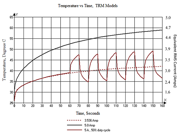
Figure 2. Temperature curves for a 5.0A, 0.05Hz waveform at 50% duty cycle (red), along with 5.0A and 3.536A curves.
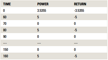
TRM offers an alternative way to look at an alternating waveform, that is, to apply current to the waveform according to a cyclical schedule supplied by the user. The schedule is provided by way of an Excel spreadsheet. An example is shown in TABLE 2. “Time” is in seconds. “Power” and “Return” are the current input and output pads, respectively, for the model. The values in the table are the current that will be applied to those pads until the next time specified. This example is for a 5.0A current (RMS value is applied for the first 60 sec.7) at a 0.05Hz frequency (after the first 60 sec.) with a 50% duty cycle.
Table 2. Cyclical Input Data for TRM Analysis
The solid red curve in Figure 2 is the resulting waveform. Its “mean” temperature is the same as that found in Figure 1, trending to about 45.4˚C.
TRM offers yet a third way to look at all this. First, we run a transient model at 5.0As (the black curve in Figure 2), which derives a “heating curve.” Then we use the PWM (Pulse Width Modulation) option found under the “Extra” menu (FIGURE 3). This modulates the heating curve with a duty cycle. Setting the “Time interval t2” and “Time interval t3” each to 10 sec. gives us a 20 sec. cycle or 0.05Hz. The 1.464W power value comes from a basic model run of 5.0As. It is the power dissipated in the trace (= I2*R).8
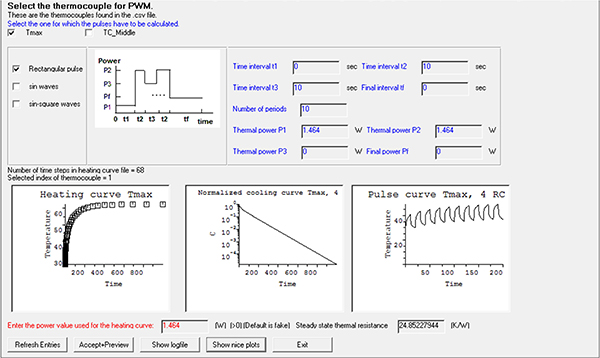
Figure 3. Setting up the PWM function in TRM.
FIGURE 4 is the resulting waveform. The shape of this waveform looks almost exactly like the waveform in Figure 2. (Technical note: The PWM approach will slightly understate the other approaches in amplitude because it does not yet take the thermal coefficient of resistivity into consideration for the calculations.5) Therefore, these latter two approaches to determining the waveform of an AC signal are equivalent, but the last approach is the easiest and most versatile, and requires minimal CPU time.
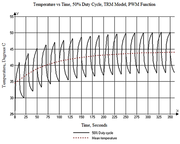
Figure 4. The resulting waveform calculation from the PWM function.
This now gives us an easy way to look at other duty cycles. For example, let’s set t2 and t3 to 5 and 20 sec., respectively (and vice versa). This gives us a frequency of 0.04Hz, at a 20% or 80% duty cycle. This results in the curves shown in FIGURE 5. TRM’s PWD function also provides the mean temperature for each cycle in this waveform. The trend-line for the mean values approaches the 33.8˚C maximum temperature for the 20% duty cycle and the 56.8˚C maximum temperature for the 80% duty cycle in Table 1.5
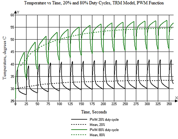
Figure 5. The resulting waveform calculation from PWM for a 0.04Hz frequency, 20% and 80% duty cycle waveforms.
So far, the TRM models seem to make some intuitive sense at lower frequencies. The PWM function will also enable us to estimate the temperatures of traces at higher frequencies. FIGURE 6 is the result from the PWM function at 100Hz, 50% duty cycle. The cycles are now so short the individual cycles are not visible, and have no effect on the result. The curve looks like the curve for a DC current at the equivalent RMS level (3.54As) and levels off at about 44˚C. This equates to a value from Figure 1 of 45.4˚C, but without the thermal coefficient of resistivity adjustment.
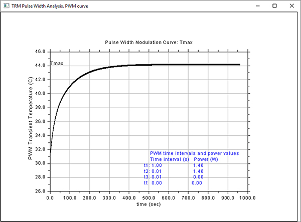
Figure 6. PWM result for a 100Hz, 50% duty cycle input current.
Preliminary Results
The conclusions so far would seem to suggest:
- The temperature of a trace is determined by the equivalent RMS value of the current driving it.
- The temperature of a trace at any duty cycle seems to be independent of frequency (at least at frequencies below where the skin effect comes into play).
Empirical verification. We had two boards left over from our via evaluation4 to use in our empirical testing. One of the traces on each board is identical to the model used above. The diagram of the test procedure is shown in FIGURE 7.
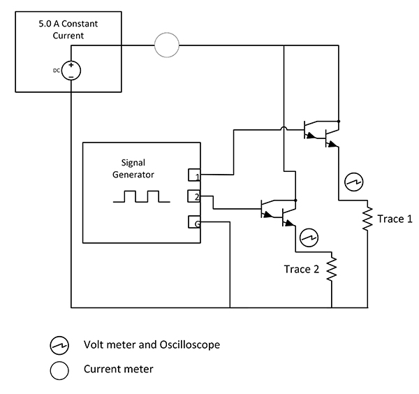
Figure 7. Diagram of empirical test setup.
A constant current generator is set to 5As. It is important the current flow not be interrupted, lest the generator output change dramatically, trying to maintain the constant current flow. Therefore, it is important to maintain a constant current from the generator, even though the current through a trace is changing. To achieve this, we used two identical test traces with current switching between them very quickly. The current was switched by a pair of Darlington transistors, each driven by a waveform generator. The waveform generator has two complementary outputs. These outputs were set to a square wave with output between 0.0 and 4.0V. The frequency was adjustable between 0.01Hz and over 20.0MHz in 0.01Hz steps. The duty cycle could be set from 0.1% to 99.9% in 0.1% steps. Current and voltage meters, and oscilloscope probes, were set where indicated. The temperature of each trace was measured with a thermocouple data logger with a sampling rate of 1.0 sec. and a resolution of 0.5˚C. The ambient environment was a typical office environment with a temperature about 26˚C.
For the first test, the duty cycle was set to 50%, and the frequency varied from 0.05 to 10,000Hz. The results are shown in Figure 8. The temperature is constant at 45˚C within the resolution of the thermocouple. This compares to the 45.4˚C temperature recorded in Table 1.
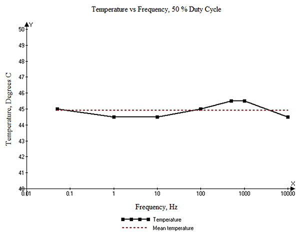
Figure 8. Temperature at 50% duty cycle as a function of frequency.
Next, we looked at the temperature as a function of duty cycle at two different frequencies, 100Hz and 10KHz. Those results are plotted in FIGURE 9. They reflect a linear relationship, within the probable experimental error. These results are consistent with the conclusions reached above with the TRM model. (See Figure 1.)
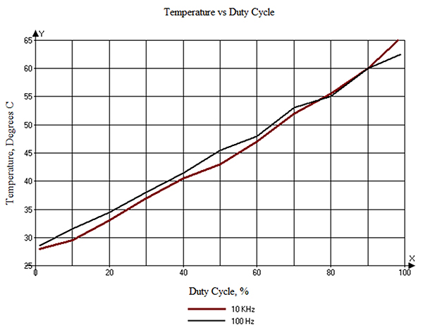
Figure 9. Temperature as a function of duty cycle.
Finally, we recorded the temperature for a 0.04Hz frequency at an 80% duty cycle (after the temperature cycles had had time to stabilize). The results are shown in FIGURE 10. For comparison, some data from the TRM PWM analysis (Figure 5) are plotted on the same axes for the same conditions. Recall the thermocouple has a 0.5˚ resolution and a 1 sec. sampling rate. The curve also reflects some “wiggles” caused by the difficulty in holding the thermocouple steady for several seconds time! Also recall the PWM analysis slightly understates the actual results because it does not take the thermal coefficient of resistivity into consideration.
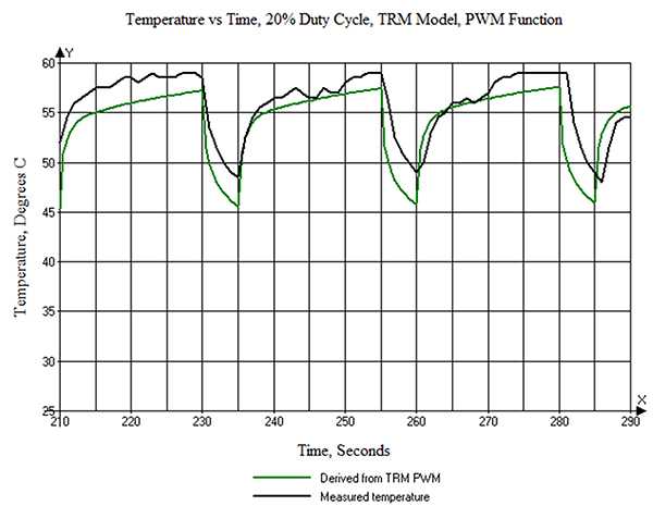
Figure 10. Temperature vs. time for a 0.04Hz, 80% duty cycle waveform.
Conclusions
It would appear we can confirm the preliminary conclusions reached above:
- The temperature of a trace is determined by the equivalent RMS value of the current driving it.
- The temperature of a trace at any frequency and duty cycle seems to be independent of frequency (at least at frequencies below where the skin effect comes into play).
Acknowledgments
The empirical measurements we made could not have been done without the help and support of Prototron Circuits (Redmond, WA, and Tucson, CA). C-Therm Technologies (Fredericton, New Brunswick) graciously provided measurements of the dielectric thermal conductivity coefficients to aid in thermal modeling.
Notes
1. See, for example, Douglas G. Brooks and Johannes Adam, “Trace Current/Temperature Relationships,” PCD&F, June 2015. See also the authors’ book, PCB Trace and Via Currents and Temperatures: The Complete Analysis, available at Amazon.com.
2. TRM (Thermal Risk Management) was created by Dr. Johannes Adam, president of Adam Research (adam-research.com). TRM was originally conceived and designed to analyze temperatures across a circuit board, taking into consideration the complete trace layout with optional Joule heating, as well as various components and their own contributions to heat generation. Learn more about TRM at adam-research.com.
3. We describe how to construct a basic TRM model in Chapter 6 of PCB Trace and Via Currents and Temperatures: The Complete Analysis.
4. Douglas G. Brooks and Johannes Adam, “Empirical Confirmation of Via Temperatures,” PCD&F, February 2016.
5. As trace temperature increases, the resistance of the trace increases (because of the thermal coefficient of resistivity). Thus, trace temperature increases even higher. TRM can take this into account in its calculations. However, this capability has not yet been programmed into the PWM module. Therefore, the PWM module tends to understate the temperature slightly. That effect is noticeable, but not large, in the temperature ranges investigated in this paper.
6. The slight “glitches” in the curve are caused by adjustments to the HTC value in the model. See Reference 3, Section 6.1. The curve should be perfectly linear.
7. Applying the RMS value for a 50% duty cycle for the first 60 sec. gets the curve “up to temperature” a little more rapidly.
8. The trace is 27 mils wide, 2.9 mils thick, and 5.9” long. It will have a resistance at 60˚ of approximately 0.063Ω if uniformly heated. I2R for 5As would therefore be approximately 1.58W. But the trace is not uniformly heated; it cools toward the pads at each end. The model calculates the total power dissipated in the trace is 1.464W.
Douglas Brooks, Ph.D., is owner of UltraCAD Design, a PCB design service bureau and author of PCB Currents: How They Flow, How They React; This email address is being protected from spambots. You need JavaScript enabled to view it.. DR. Johannes Adam, Ph.D., CID, is founder of ADAM Research, a technical consultant for electronics companies, a software developer, and the author of the Thermal Risk Management simulation program.