Do analog waveforms follow the same relationship as other signals?
In a recent article,2 we looked at the relationship between trace current and temperature for pulses that propagated through the trace. That type of circuit was relatively easy to construct because a constant current was either applied to the trace or it wasn’t. That is, it was switched “on” and “off.” In effect, the test currents were digital, switched currents.
The results were not unexpected:
1. The effective current applied by the switched pulse was the RMS (root mean square) current, and
2. The temperature was independent of frequency (at least over the tested range).
But a question still remains: What about analog AC currents? What about sine or triangular waveforms? This article looks at the slightly more complicated topic of analog waveforms to see if the same conclusions apply.
Test circuit. The first problem is how to apply an analog signal of known, repeatable current level through a trace at a significant enough current to heat the trace. To accomplish this, the circuit shown in FIGURE 1 was created. A waveform generator applied one of three signal types to the base of the Darlington transistor. That resulted in a current through the trace controlled by the current through the collector. That current was supplied by a 10.0V constant voltage generator through a 1.05Ω resistor (with a very low temperature coefficient). The current through the trace is derived as:
Current = (10.0 - voltage at collector)/1.05
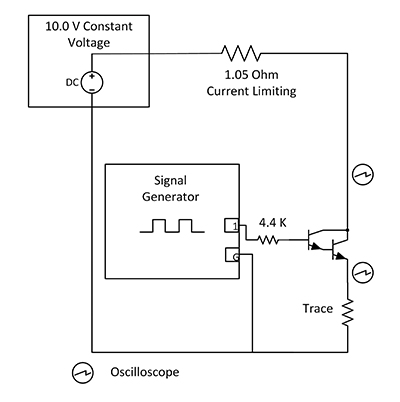
Figure 1. Test schematic.
The waveform generator settings were extremely flexible. The output voltage could be set from 0.0 to 10.0V. The frequency could be set from 0.01Hz to over 20MHz. And the signal DC offset could be set from -10.0 to +10.0V DC. Three waveforms were employed during this analysis: sine, triangle (actually sawtooth) and square. The duty cycle for the square and triangular waveforms could be set from 0.0 to 99.9%. The duty cycle for the triangular waveform was set at 99.9% (sawtooth), and the duty cycles for the square waves were set at 50%, 75% and 99%. Output levels were set to result in large output currents, but not large enough to switch the transistor off, nor to bring it into saturation. Samples of the waveform generator output waveforms are shown in FIGURE 2. The generator waveforms exhibited no measurable distortion.
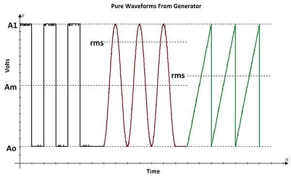
Figure 2. Waveform generator outputs.
RMS signal levels. Next, we need to consider how to calculate the rms values of the signals.3 There are some reference lines drawn on Figure 2:
A1 Peak voltage
A0 Minimum voltage
Am Average voltage; i.e., Am = (A1-A0)/2)
If we ignore any DC offset, the rms value of a simple square wave is simply its peak voltage, shown as (A1-Am) in Figure 2. But if the square wave has a duty cycle other than 50%, it looks more like the pulse train in Part 1 of this series.2 The rms value of the pulse train is its peak value multiplied by the square root of the duty cycle, or (A1-Ao)*SQRT(duty cycle).
Similarly, if we ignore any DC offset, the rms voltage of a simple sine wave is .707*peak, or .707*(A1-Am) in Figure 2. And, ignoring any DC offset, the rms value of a simple triangular (or sawtooth) waveform is 0.577*peak, or .577*(A1-A0) in Figure 2.
If there is a DC offset, the rms values are calculated as follows:
Let rms = the rms value of the simple waveform.
Let dc = the dc offset (Am for the simple square wave and the sine wave, Ao for the sawtooth wave and the pulse train.)
Then the rms value of the offset waveform is
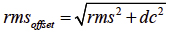
Nonlinearities. But there can be a problem in a practical circuit. The circuit (transistor) is non-linear over the range of current applied here. For example, FIGURE 3 shows the resulting sawtooth waveform. The degree of non-linearity is obvious.
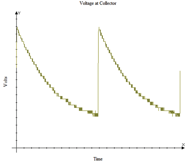
Figure 3. Sawtooth voltage waveform vs time at the collector.
The oscilloscope used in this analysis was a PicoScope model 2204A digital scope whose output can be saved to a computer file. The scope also has the ability to calculate the “True RMS” voltage (as well as the DC average, and many other measures) of the waveform under evaluation. Therefore, we are freed from having to manually calculate the rms value.
But then, there is another problem. In our circuit, high voltages at the collector correspond to low currents through the trace, and low voltages at the collector correspond with high currents through the trace. The root-mean-square calculation tends to bias the results to the higher values, in this case the opposite of what we want. Fortunately, the scope can output a data file, which can be imported into an Excel spreadsheet. The data can be corrected and the rms value calculated by the spreadsheet.4
Results. The trace used in this analysis was one of the traces on a test board used in a previous study.5 It was a 100 mil wide, 0.5oz., 6" long trace. The resulting summary data are shown in TABLE 1 and graphed in FIGURE 4. These results were obtained at a frequency of 100Hz.6 The black line in Figure 4 is the current/temperature relationship for the trace with DC current applied. These results are consistent with prior results; i.e., the effective current for current/temperature analyses of ac waveforms is the rms value of the current.
Table 1. Summary Results of Testing
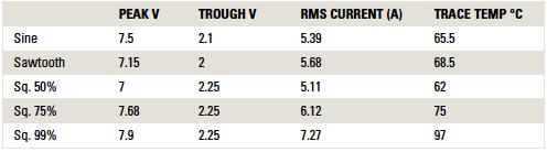
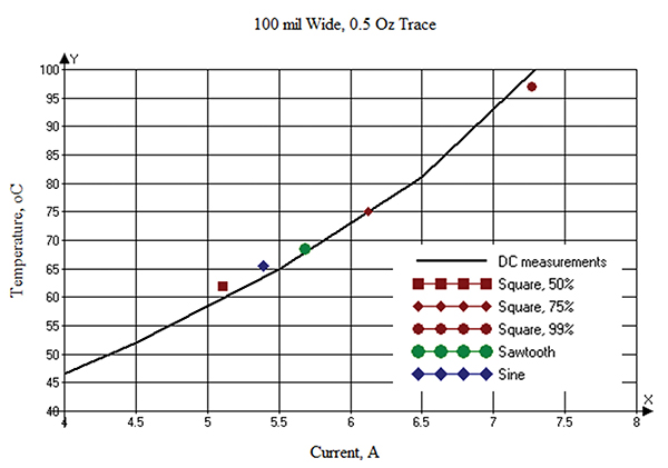
Figure 4. Graph of summary results.
When applying the signals to the trace, we also varied the frequency from 0.5Hz to 1,000Hz. The temperatures remained constant with frequency within the measurement accuracy of the study (as expected). (At frequencies significantly above 5,000Hz, our test setup became unstable.)
Conclusions
We conclude the results of this analysis are consistent with the prior results:
1. The effective current of an analog ac waveform is the RMS (root mean square) current, and
2. The temperature of an analog ac waveform is independent of frequency (at least over the tested range).
Acknowledgments
The empirical measurements could not have been done without the help and support of Prototron Circuits (Redmond, WA, and Tucson, CA).
Notes
1. Douglas G. Brooks and Johannes Adam, “PCB Trace and Via Temperatures and Currents: The Complete Analysis,” CreateSpace Independent Publishing Platform, March 2016.
2. Douglas G. Brooks and Johannes Adam, “How AC Currents Affect PCB Trace Temperatures,” PCD&F, September 2016.
3. See https://en.wikipedia.org/wiki/Root_mean_square.
4. There are approximately 900 data samples per cycle in our waveforms. The Excel formula for calculating rms is = SQRT(SUMSQ(A1:A10)/COUNTA(A1:A10)), where A1:A10 is the data range of interest.
5. Douglas G. Brooks, “Empirical Results of Fusing Tests,” PCD&F, January 2016.
6. At frequencies above about 10Hz, the thermal inertia is such that the temperature does not change much within the cycle.
Douglas Brooks, Ph.D., is owner of UltraCAD Design, a PCB design service bureau and author of PCB Currents: How They Flow, How They React; This email address is being protected from spambots. You need JavaScript enabled to view it.. Dr. Johannes Adam, Ph.D., CID, is founder of ADAM Research, a technical consultant for electronics companies, a software developer, and the author of the Thermal Risk Management simulation program.